Arithmethic - Geometric sequences

The two simplest sequences to work with are arithmetic and geometric sequences. An arithmetic sequence goes from one term to the next by always adding (or subtracting) the same value. For instance, 2, 5, 8, 11, 14,... and 7, 3, –1, –5,... are arithmetic, since you add 3 and subtract 4, respectively, at each step. A geometric sequence goes from one term to the next by always multiplying (or dividing) by the same value. So 1, 2, 4, 8, 16,... and 81, 27, 9, 3, 1, 1/3,... are geometric, since you multiply by2 and divide by 3, respectively, at each step.
The number added (or subtracted) at each stage of an arithmetic sequence is called the "common difference" d, because if you subtract (find the difference of) successive terms, you'll always get this common value. The number multiplied (or divided) at each stage of a geometric sequence is called the "common ratio" r, because if you divide (find the ratio of) successive terms, you'll always get this common value.

• Find the common difference and the next term of the following sequence:
3, 11, 19, 27, 35,...
To find the common difference, I have to subtract a pair of terms. It doesn't matter which pair I pick, as long as they're right next to each other:

11 – 3 = 8
19 – 11 = 8
27 – 19 = 8
35 – 27 = 8
The difference is always 8, so d = 8. Then the next term is 35 + 8 = 43.

• Find the common ratio and the seventh term of the following sequence:
2/9, 2/3, 2, 6, 18,...
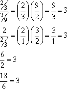
To find the common ratio, I have to divide a pair of terms. It doesn't matter which pair I pick, as long as they're right next to each other:

The ratio is always 3, so r = 3. Then the sixth term is (18)(3) = 54 and the seventh term is(54)(3) = 162.

---

Since arithmetic and geometric sequences are so nice and regular, they have formulas.
For arithmetic sequences, the common difference is d, and the first term a₁ is often referred to simply as "a". Since you get the next term by adding the common difference, the value of a₂ is just a + d. The third term is a₃ = (a + d) + d = a + 2d. The fourth term is a₄ = (a + 2d) + d = a + 3d. Following this pattern, the n-th term a_n will have the form a_n = a + (n – 1)d.
For geometric sequences, the common ratio is r, and the first term a₁ is often referred to simply as"a". Since you get the next term by multiplying by the common ratio, the value of a₂ is just ar. The third term is a₃ = r(ar) = ar². The fourth term is a₄ = r(ar²) = ar³. Following this pattern, the n-th term a_n will have the form a_n = ar^{(n – 1)}.

• Find the tenth term and the n-th term of the following sequence:
1/2, 1, 2, 4, 8,...
The differences don't match: 2 – 1 = 1, but 4 – 2 = 2. So this isn't an arithmetic sequence. On the other hand, the ratios are the same: 2 ÷ 1 = 2, 4 ÷ 2 = 2, 8 ÷ 4 = 2. So this is a geometric sequence with common ratio r = 2 and a = 1/2. To find the tenth and n-th terms, I can just plug into the formula a_n = ar^{(n – 1)}:

a_n = (1/2) 2^n–1 
a₁₀ = (1/2) 2^10–1 = (1/2) 2⁹ = (1/2)(512) = 256

• Find the n-th term and the first three terms of the arithmetic sequence having a₆ = 5 andd = 3/2.
The n-th term of an arithmetic sequence is of the form a_n = a + (n – 1)d. In this case, that formula gives me a₆ = a + (6 – 1)(3/2) = 5. Solving this formula for the value of the first term of the sequence, I get a = –5/2. Then:

a₁ = –5/2, a₂ = –5/2 + 3/2 = –1, a₃ = –1 + 3/2 = 1/2,
and a_n = –5/2 + (n – 1)(3/2)

• Find the n-th term and the first three terms of the arithmetic sequence having a₄ = 93 anda₈ = 65.
Since a₄ and a₈ are four places apart, then I know from the definition of an arithmetic sequence that a₈ = a₄ + 4d. Using this, I can then solve for the common difference d:

65 = 93 + 4d 
–28 = 4d 
–7 = d
Also, I know that a₄ = a + (4 – 1)d, so, using the value I just found for d, I can find the value of the first term a:

93 = a + 3(–7) 
93 + 21 = a 
114 = a
Once I have the value of the first term and the value of the common difference, I can plug-n-chug to find the values of the first three terms and the general form of the n-th term:

a₁ = 114, a₂ = 114 – 7 = 107, a₃ = 107 – 7 = 100
a_n = 114 + (n – 1)(–7)

Suppose a1, a2, a3, …. is an A.P. and b1, b2, b3, …… is a G.P. Then the sequence a1b1, a2b2, …, anbn is said to be an arithmetic-geometric progression. An arithmetic-geometric progression is of the form ab, (a+d)br, (a + 2d)br2, (a + 3d)br3, ……

Its sum Sn to n terms is given by

Sn = ab + (a+d)br + (a+2d)br2 +……+ (a+(n–2)d)brn–2 + (a+(n–1)d)brn–1.

Multiply both sides by r, so that

rSn = abr+(a+d)br2+…+(a+(n–3)d)brn–2+(a+(n–2)d)brn–1+(a+(n–1)d)brn.

Subtracting we get

(1 – r)Sn = ab + dbr + dbr2 +…+ dbrn–2 + dbrn–1 – (a+(n–1)d)brn.

        = ab + dbr(1–rn–1)/(1–r) (a+(n–1)d)brn

        ⇒ Sn = ab/1–r + dbr(1–rn–1)/(1–r)2 – (a+(n–1)d)brn/1–r.

If –1 < r < 1, the sum of the infinite number of terms of the progression is

        limn→∞ Sn = ab/1–r + dbr/(1–r)2.

Mode

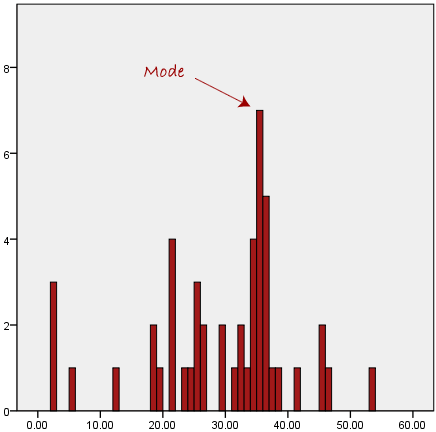
The mode is the most frequent score in our data set. On a histogram it represents the highest bar in a bar chart or histogram. You can, therefore, sometimes consider the mode as being the most popular option. An example of a mode is presented below:

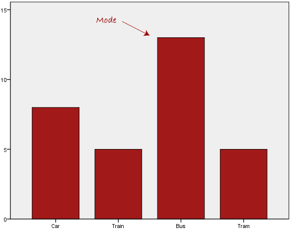
Normally, the mode is used for categorical data where we wish to know which is the most common category, as illustrated below:

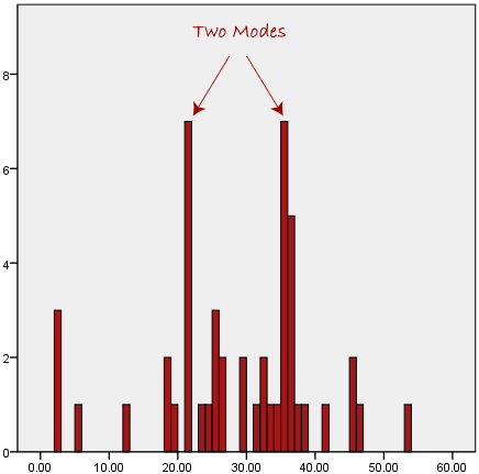
We can see above that the most common form of transport, in this particular data set, is the bus. However, one of the problems with the mode is that it is not unique, so it leaves us with problems when we have two or more values that share the highest frequency, such as below:

We are now stuck as to which mode best describes the central tendency of the data. This is particularly problematic when we have continuous data because we are more likely not to have any one value that is more frequent than the other. For example, consider measuring 30 peoples' weight (to the nearest 0.1 kg). How likely is it that we will find two or more people with exactly the same weight (e.g., 67.4 kg)? The answer, is probably very unlikely - many people might be close, but with such a small sample (30 people) and a large range of possible weights, you are unlikely to find two people with exactly the same weight; that is, to the nearest 0.1 kg. This is why the mode is very rarely used with continuous data.

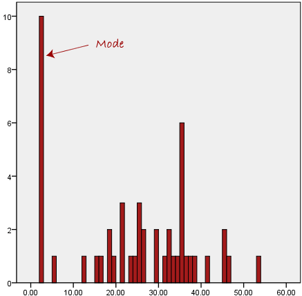
Another problem with the mode is that it will not provide us with a very good measure of central tendency when the most common mark is far away from the rest of the data in the data set, as depicted in the diagram below:

In the above diagram the mode has a value of 2. We can clearly see, however, that the mode is not representative of the data, which is mostly concentrated around the 20 to 30 value range. To use the mode to describe the central tendency of this data set would be misleading.

Skewed Distributions and the Mean and Median

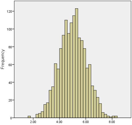
We often test whether our data is normally distributed because this is a common assumption underlying many statistical tests. An example of a normally distributed set of data is presented below:

When you have a normally distributed sample you can legitimately use both the mean or the median as your measure of central tendency. In fact, in any symmetrical distribution the mean, median and mode are equal. However, in this situation, the mean is widely preferred as the best measure of central tendency because it is the measure that includes all the values in the data set for its calculation, and any change in any of the scores will affect the value of the mean. This is not the case with the median or mode.

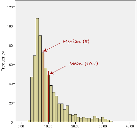
However, when our data is skewed, for example, as with the right-skewed data set below:

we find that the mean is being dragged in the direct of the skew. In these situations, the median is generally considered to be the best representative of the central location of the data. The more skewed the distribution, the greater the difference between the median and mean, and the greater emphasis should be placed on using the median as opposed to the mean. A classic example of the above right-skewed distribution is income (salary), where higher-earners provide a false representation of the typical income if expressed as a mean and not a median.

If dealing with a normal distribution, and tests of normality show that the data is non-normal, it is customary to use the median instead of the mean. However, this is more a rule of thumb than a strict guideline. Sometimes, researchers wish to report the mean of a skewed distribution if the median and mean are not appreciably different (a subjective assessment), and if it allows easier comparisons to previous research to be made.

Summary of when to use the mean, median and mode

Please use the following summary table to know what the best measure of central tendency is with respect to the different types of variable.

Type of Variable	Best measure of central tendency
Nominal	Mode
Ordinal	Median
Interval/Ratio (not skewed)	Mean
Interval/Ratio (skewed)	Median

Median

The median is the middle score for a set of data that has been arranged in order of magnitude. The median is less affected by outliers and skewed data. In order to calculate the median, suppose we have the data below:

65

55

89

56

35

14

56

55

87

45

92

We first need to rearrange that data into order of magnitude (smallest first):

14

35

45

55

55

56

56

65

87

89

92

Our median mark is the middle mark - in this case, 56 (highlighted in bold). It is the middle mark because there are 5 scores before it and 5 scores after it. This works fine when you have an odd number of scores, but what happens when you have an even number of scores? What if you had only 10 scores? Well, you simply have to take the middle two scores and average the result. So, if we look at the example below:

65

55

89

56

35

14

56

55

87

45

We again rearrange that data into order of magnitude (smallest first):

14

35

45

55

55

56

56

65

87

89

Only now we have to take the 5th and 6th score in our data set and average them to get a median of 55.5.

Measure of Central Tendency

Introduction

A measure of central tendency is a single value that attempts to describe a set of data by identifying the central position within that set of data. As such, measures of central tendency are sometimes called measures of central location. They are also classed as summary statistics. The mean (often called the average) is most likely the measure of central tendency that you are most familiar with, but there are others, such as the median and the mode.

The mean, median and mode are all valid measures of central tendency, but under different conditions, some measures of central tendency become more appropriate to use than others. In the following sections, we will look at the mean, mode and median, and learn how to calculate them and under what conditions they are most appropriate to be used.

Mean (Arithmetic)

The mean (or average) is the most popular and well known measure of central tendency. It can be used with both discrete and continuous data, although its use is most often with continuous data (see our Types of Variable guide for data types). The mean is equal to the sum of all the values in the data set divided by the number of values in the data set. So, if we have n values in a data set and they have values x₁, x₂, ..., x_n, the sample mean, usually denoted by  (pronounced x bar), is:

This formula is usually written in a slightly different manner using the Greek capitol letter, , pronounced "sigma", which means "sum of...":

You may have noticed that the above formula refers to the sample mean. So, why have we called it a sample mean? This is because, in statistics, samples and populations have very different meanings and these differences are very important, even if, in the case of the mean, they are calculated in the same way. To acknowledge that we are calculating the population mean and not the sample mean, we use the Greek lower case letter "mu", denoted as µ:

The mean is essentially a model of your data set. It is the value that is most common. You will notice, however, that the mean is not often one of the actual values that you have observed in your data set. However, one of its important properties is that it minimises error in the prediction of any one value in your data set. That is, it is the value that produces the lowest amount of error from all other values in the data set.

An important property of the mean is that it includes every value in your data set as part of the calculation. In addition, the mean is the only measure of central tendency where the sum of the deviations of each value from the mean is always zero.

When not to use the mean

The mean has one main disadvantage: it is particularly susceptible to the influence of outliers. These are values that are unusual compared to the rest of the data set by being especially small or large in numerical value. For example, consider the wages of staff at a factory below:

Staff	1	2	3	4	5	6	7	8	9	10
Salary	15k	18k	16k	14k	15k	15k	12k	17k	90k	95k

The mean salary for these ten staff is $30.7k. However, inspecting the raw data suggests that this mean value might not be the best way to accurately reflect the typical salary of a worker, as most workers have salaries in the $12k to 18k range. The mean is being skewed by the two large salaries. Therefore, in this situation, we would like to have a better measure of central tendency. As we will find out later, taking the median would be a better measure of central tendency in this situation.

Another time when we usually prefer the median over the mean (or mode) is when our data is skewed (i.e., the frequency distribution for our data is skewed). If we consider the normal distribution - as this is the most frequently assessed in statistics - when the data is perfectly normal, the mean, median and mode are identical. Moreover, they all represent the most typical value in the data set. However, as the data becomes skewed the mean loses its ability to provide the best central location for the data because the skewed data is dragging it away from the typical value. However, the median best retains this position and is not as strongly influenced by the skewed values. This is explained in more detail in the skewed distribution section later in this guide.

Probability

How likely something is to happen.

Many events can't be predicted with total certainty. The best we can say is how likely they are to happen, using the idea of probability.

Tossing a Coin  When a coin is tossed, there are two possible outcomes: heads (H) or tails (T) We say that the probability of the coin landing H is ½. And the probability of the coin landing T is ½.

Throwing Dice  When a single die is thrown, there are six possible outcomes: 1, 2, 3, 4, 5, 6. The probability of any one of them is 1/6.

Probability 

In general:

Probability of an event happening = Number of ways it can happenTotal number of outcomes

Example: the chances of rolling a "4" with a die

Number of ways it can happen: 1 (there is only 1 face with a "4" on it)

Total number of outcomes: 6 (there are 6 faces altogether)

So the probability = 16

Example: there are 5 marbles in a bag: 4 are blue, and 1 is red. What is the probability that a blue marble gets picked?

Number of ways it can happen: 4 (there are 4 blues)

Total number of outcomes: 5 (there are 5 marbles in total)

So the probability = 45 = 0.8

Probability Line

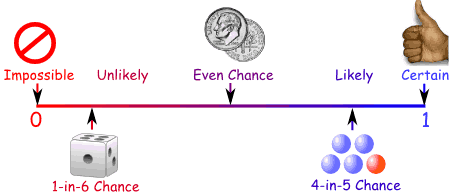
We can show probability on a Probability Line:

Probability is always between 0 and 1

Probability is Just a Guide

Probability does not tell us exactly what will happen, it is just a guide

Example: toss a coin 100 times, how many Heads will come up?

Probability says that heads have a ½ chance, so we can expect 50 Heads.

But when we actually try it we might get 48 heads, or 55 heads ... or anything really, but in most cases it will be a number near 50.

Linear Programming

Linear programming (LP) (also called linear optimization) is a method to achieve the best outcome (such as maximum profit or lowest cost) in a mathematical model whose requirements are represented by linear relationships. Linear programming is a special case of mathematical programming (mathematical optimization).

More formally, linear programming is a technique for the optimization of a linear objective function, subject to linear equality and linear inequality constraints. Its feasible region is a convex polytope, which is a set defined as the intersection of finitely many half spaces, each of which is defined by a linear inequality. Its objective function is a real-valued affine (linear) function defined on this polyhedron. A linear programming algorithm finds a point in the polyhedron where this function has the smallest (or largest) value if such a point exists.

Linear programs are problems that can be expressed in canonical form as

${\displaystyle {\begin{aligned}&{\text{maximize}}&&\mathbf {c} ^{\mathrm {T} }\mathbf {x} \\&{\text{subject to}}&&A\mathbf {x} \leq \mathbf {b} \\&{\text{and}}&&\mathbf {x} \geq \mathbf {0} \end{aligned}}}$

where x represents the vector of variables (to be determined), c and b are vectors of (known) coefficients, A is a (known) matrix of coefficients, and ${\displaystyle (\cdot )^{\mathrm {T} }}$ is the matrix transpose. The expression to be maximized or minimized is called the objective function (c^Tx in this case). The inequalities Ax ≤ b and x ≥ 0 are the constraints which specify a convex polytope over which the objective function is to be optimized. In this context, two vectors are comparable when they have the same dimensions. If every entry in the first is less-than or equal-to the corresponding entry in the second then we can say the first vector is less-than or equal-to the second vector.

Linear programming can be applied to various fields of study. It is widely used in business and economics, and is also utilized for some engineering problems. Industries that use linear programming models include transportation, energy, telecommunications, and manufacturing. It has proved useful in modeling diverse types of problems in planning, routing, scheduling, assignment, and design.

Linear Inequalities

Solving linear inequalities

The graph of a linear inequality in one variable is a number line. Use an open circle for < and > and a closed circle for ≤ and ≥.

The graph for x > -3

The graph for x ≥ 2

Inequalities that have the same solution are called equivalent. There are properties of inequalities as well as there were properties of equality. All the properties below are also true for inequalities involving ≥ and ≤.

The addition property of inequality says that adding the same number to each side of the inequality produces an equivalent inequality

Ifx>y,thenx+z>y+z$$Ifx>y,thenx+z>y+z$$

Ifx<y,thenx+z<y+z$$Ifx<y,thenx+z<y+z$$

The subtraction property of inequality tells us that subtracting the same number from both sides of an inequality gives an equivalent inequality.

Ifx>y,thenx−z>y−z$$Ifx>y,thenx-z>y-z$$

Ifx<y,thenx−z<y−z$$Ifx<y,thenx-z<y-z$$

The multiplication property of inequality tells us that multiplication on both sides of an inequality with a positive number produces an equivalent inequality.

Ifx>yandz>0,thenxz>yz$$Ifx>yandz>0,thenxz>yz$$

Ifx<yandz>0,thenxz<yz$$Ifx<yandz>0,thenxz<yz$$

Multiplication in each side of an inequality with a negative number on the other hand does not produce an equivalent inequality unless we also reverse the direction of the inequality symbol

Ifx>yandz<0,thenxz<yz$$Ifx>yandz<0,thenxz<yz$$

Ifx<yandz<0,thenxz>yz$$Ifx<yandz<0,thenxz>yz$$

The same goes for the division property of inequality.

Division of both sides of an inequality with a positive number produces an equivalent inequality.

Ifx>yandz>0,thenxz>yz$$Ifx>yandz>0,then\frac{x}{z}>\frac{y}{z}$$

Ifx<yandz>0,thenxz<yz$$Ifx<yandz>0,then\frac{x}{z}<\frac{y}{z}$$

And division on both sides of an inequality with a negative number produces an equivalent inequality if the inequality symbol is reversed.

Ifx>yandz<0,thenxz<yz$$Ifx>yandz<0,then\frac{x}{z}<\frac{y}{z}$$

Ifx<yandz<0,thenxz>yz$$Ifx<yandz<0,then\frac{x}{z}>\frac{y}{z}$$

To solve a multi-step inequality you do as you did when solving multi-step equations. Take one thing at the time preferably beginning by isolating the variable from the constants. When solving multi-step inequalities it is important to not forget to reverse the inequality sign when multiplying or dividing with negative numbers.